Cassandra
A NoSQL wide-column database
Paul Krzyzanowski
November 5, 2021
Goal: How can we build an ultra-high performance, low-latency multi-table database that can grow incrementally to handle massive-scale data?
Introduction
Cassandra is a large-scale open-source NoSQL wide-column distributed database. It was developed at Facebook and its design was influenced by Amazon Dynamo and Google Bigtable.
Cassandra was initially developed to handle inbox searches at Facebook. This involves storing reverse indices of Facebook messages that users send and receive. A reverse index maps message contents to messages. That is, the system can look up a word and find all messages that contain text with that word in it. Facebook was growing rapidly and it was clear that not only was a high-performing solution needed but its design had to be able to scale as the amount of data and number of users grew. The key goals of Cassandra were high performance, incremental scalability, and high availability. Since the CAP theorem tells us we must choose between consistency and availability if a network partition occurs, Cassandra opted for high availability at the expense of consistency, implementing an eventually consistent model. This also helps with performance since there is no need to take and release locks across all nodes that store replicas of data that’s being modified.
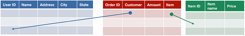
Cassandra is an example of a NoSQL database. SQL stands for Structured Query Language and is the de facto standard language for interacting with relational databases. Relational databases are characterized by supporting multiple tables where each table has a set of fields that are defined when that table is created. Each row of the table is identified by a unique key and the database implements indexing structures that enable rapid lookup of the row by the key. Some fields in a row may contain reference to keys that belong to other tables. These “relations” are called foreign keys. For instance, a table of product orders may be indexed by an order ID (the key). Each row might contain a foreign key that refers to the user that placed the order in a customers table as well a foreign key for the item description in an Items table.
With a SQL — or relational — database, we expect ACID semantics: data access that is atomic, consistent, isolated, and durable. This means that if a row is being modified by a transaction, no other transaction can access that data. If multiple tables are involved in a transaction, all rows that area accessed by those tables need to be locked so other transactions cannot modify the data. If any data is replicated (which we want to do for high availability), all replicas must be locked so no transactions access old data. We looked at this in some detail when we looked at commit protocols and concurrency control.
A NoSQL database refers to an eventually-consistent, non-relational database. ACID semantics no longer apply. These databases choose high availability over strong consistency and there is a chance that some transactions may access stale data. The non-relational aspect of a NoSQL database means that the database does not define foreign keys that create relationships among tables. A field might contain data that is used to look up a row in another table, but the database is oblivious to this function and will not do any integrity checking or lock the affected rows during a transaction.
NoSQL databases are often designed as wide-column data stores. Traditional relational databases comprise tables that have a small, fixed set of fields, or columns, that are defined when the table is created (e.g., user ID, name, address, city, state, country, phone). In wide-column data stores, a row may have an arbitrary number of columns and columns may be created dynamically after the tables are created. The only columns that are expected to be present are the key (which is essential to identify a row uniquely and look up a row efficiently) and any columns that user software deems to be mandatory for the application.
The concept of wide columns changes the way columns are used in a data store. With a traditional database, the programmer is aware of the columns (fields) within a table. A wide-column table, on the other hand, may contain different columns for different rows and the programmer may need to iterate over their names.
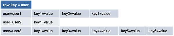
For example a user might have multiple phone numbers that, instead of being stored in a separate table with foreign keys that identify the owner of each number, are co-located with the user’s information. Each number is a new column (e.g., phone-1, phone-2, …). There’s also no limit to the number of columns in a row. As we saw with Bigtable, columns might be a list of URLs. In the Bigtable example, a URL of a web page serves as a row key but column names within the URL have names of URLs that contain links to that page and the value of each of those columns contains the link text that appears within the page. We can also consider a related example where a row key identifies a user and each column name is a URL that the user visited and its value is the time of the visit. This is a powerful departure from conventional database fields because the column name itself may be treated as a form of value: by iterating over the columns, one can obtain a list of URLs and then look up their associated value (e.g., link text or time of visit).
Wide-column data stores such as Bigtable and Cassandra essentially have no limit on the number of columns that can be associated with a row. In the case of Cassandra, the limit is essentially the storage capacity of the node.
Cassandra Goals
Cassandra had several goals in its design:
- Because high availability was crucial, there had to be no single point of failure. Bigtable used a central coordinator. If that coordinator died, a new coordinator could start up and discover which tablet servers were responsible for which tablets … and also discover which tablets need to be assigned to tablet servers. This was possible because key information was stored in Chubby, a replicated lock manager and small object store (which can hold critical configuration data) and all Bigtable data was stored in the Google File System (GFS), which replicates its data for fault tolerance. Cassandra, on the other hand, similar to Amazon Dynamo, opted not to use a central coordinator and not to use an underlying distributed file system.
- High performance was critical, so latency must be kept to a minimum. Cassandra’s design uses a distributed hash table (DHT) similar to Amazon Dynamo (which, in turn, is similar to Chord). Any node in Cassandra might receive a query and the hope is that the node will be able to directly forward the query to the node that is responsible for the data.
- Like Google, Facebook realized that economics favor the use of commodity hardware: standard PCs running Linux instead of more expensive fault-tolerant systems. Statistically, in a large-scale environment, something will always be failing. It’s just a question of how often but that does not matter as much if the system must be designed for high availability.
- Facebook was growing rapidly, so the service must be able to scale as more nodes are added. Cassandra should run well on a single machine as well as on a network of thousands of machines.
- Similar to Dynamo, Cassandra would allow the amount of replication and the number of reads and writes that replicas must acknowledge be configurable. In addition, because entire racks of computers or entire data centers may lose connectivity, replicated data can be configured to be spread across racks and across multiple data centers to ensure high availability.
- Queries are expected to be based on a key. That is, the user identifies a specific row by providing a unique key that identifies it (e.g., user ID). Given that, the query can then modify columns, iterate over columns, insert a new column, or query the value of a specific column.
- Like Bigtable, Cassandra would be designed as a wide-column database. Each row within a table might have wildly different columns and the columns may be of different data types. There would effectively be no limit to the number of columns that a row may have.
- Finally, to make the system easy to use, Cassandra would support an interpreted query language that is vaguely similar to SQL, which is used in relational databases. Cassandra’s query language is, of course, CQL: Cassandra Query Language.
Cassandra deployment environment
Cassandra is designed for small to huge-scale deployments. Large-scale deployments may comprise tens or hundreds of thousands of machines (nodes1) and may be spread across multiple data centers. Each of these computers may accept and process queries from clients and together they form a Cassandra cluster. Each of these computers also stores part of the Cassandra database. As we will see later, the computers discover each other’s presence and arrange themselves in a logical ring just like computers did in a Chord or Amazon Dynamo distributed hash table (DHT). This ring is traversed clockwise to determine which machines store replicas of data.
A Cassandra deployment might be spread out across multiple data centers. Each data center represents a single physical location: a building.
A data center contains multiple racks of computers. Data centers vary tremendously in size. Small ones may have a few hundred racks while a large data center may have over 15,000 racks of computers.
A rack within a data center is a structure that houses a bunch of computers. Again, the number of computers per rack varies based on the size of the computers and their storage. Rack sizes are measured in “units” termed “U”. Each unit is approximately 1.75 inches tall and a rack can typically hold 42 1U computers or 74 ½U computers.
The latency for two computers to communicate is lowest when both machines are in the same rack. That way, communication only needs to flow through one ethernet switch and relatively short cables. Between racks, we have a longer physical distance and at least three switches, so latency increases. Between data centers, we might have vast distances, shared bandwidth, and may have to go through multiple routers (companies such as Google and Facebook can afford dedicated connections between some data centers but, of course, each data center is not connected to every other one).
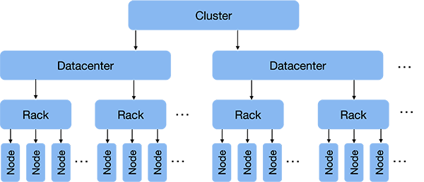
The reason that Cassandra administrators need to be aware of this environment is to be able to make intelligent availability decisions. Latency will be lowest if all – or most – of the systems are within one rack. However, if the power supply for that rack or its ethernet switch dies or gets disconnected, the entire rack of computers will be unreachable. It is safer if data is replicated onto some computer outside of the rack. Similarly, an entire data center might lose power or connectivity (or be destroyed). Hence, for high availability, it is useful to further replicate data outside of one data center even if it takes more time to do so.
Cassandra data hierarchy
Now let’s take a look at the programmer’s view of how data is stored within Cassandra before we look at how it is really stored. As with Amazon Dynamo or Google Bigtable, programmers have the abstraction of talking to a single database and don’t have to be concerned with the individual servers and where data is actually stored.
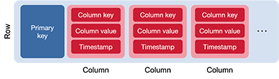
Columns
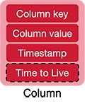
The basic unit of data storage in Cassandra is the column. A column is a set of {name, value} data. The name can be queried to find the value. Values are assigned a type and Cassandra supports a variety of data types that include:
text,varchar,ascii: UTF8 (Unicode) or ASCII character stringstinyint,smallint,int,bigint: 8-bit, 16-bit, 32-bit, and 64-bit signed integersblob: arbitrary bytesboolean: true/falsecounter: a 64-bit signed counter (values that can only be incremented or decremented)date: a date without a timetime: a time without a datetimestamp: a timestamp with millisecond precision (number of milliseconds since January 1 1970 00:00:00 GMT)decimal: variable-precision decimal numbersvarint: variable precision integersfloat,double: 32-bit and 64-bit floating point numbersduration: a duration with nanosecond precision (number of months, days, and nanoseconds)inet: an IPv4 or IPv6 address
A column can also contain a collection of data. Cassandra supports three types: a set, a list, and a map. A set is a group of elements with unique values. Items are stored unordered, there will be no duplicates, and results are sorted when queried. A list is similar to a set but the items in the list do not need to be unique and element positions have meaning. Finally, a map allows the value of a column to be a sequence of key-value pairs.
In addition to a name and value, a column stores a timestamp. The timestamp is generated by the client when the data is inserted and is used by Cassandra to resolve conflicts among replicas if there were concurrent updates. Cassandra assumes that all clocks are synchronized. Optionally, a column may be given an expiration timestamp, called a time to live. The data is not guaranteed to be deleted after the expiration time but serves as an indication that it can be deleted during scheduled compaction jobs.
Rows
A column is simply key-value data. Related columns are assembled into rows. A row is an ordered collection of columns that is identified by a key. Since Cassandra is a wide-column data store, the set of columns in a row is not preordained and new columns can be added dynamically to any row. The collection of columns in one row may be dramatically different from those in another row. If we think of the collection of rows and columns as a table (a grid), there will be cases where the columns are very sparse: many rows will not have any values for those columns.
Just like with Bigtable, all the data for a row is stored within a single file along with other rows. In the case of Cassandra, since there is no shared distributed file system and each node has its own storage, all the data for a row must fit within the node that stores that row.
Keys
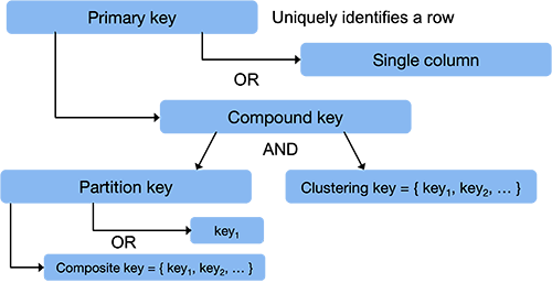
Each row in a Cassandra database is identified by a unique primary key. A query for this key allows Casandra to locate that row and provide column value that have been associated with the row. A primary key is a single or multi-column value that uniquely identifies a row. It also determines the overall sorting of data.
In the simplest case, a primary key is simply the name of a single column. In this case, it serves as the partition key. Cassandra hashes this with a consistent hash function and the resulting value is used to identify the node that stores that row of data. The choice of a partition key is where the programmer makes a conscious decision on what data should be stored on the same machine.
For example, suppose we have a database of McDonald’s restaurants around the world and each restaurant has a unique restaurant ID number. Each row contains data about a specific restaurant. If the partition key is the restaurant ID, then we expect the the set of restaurants to end up uniformly distributed throughout the machines in the cluster since we expect their hash values to be randomly distributed throughout the range of all possible hash values. This might not be the behavior we want since it might degrade query performance if applications typically do a lot of geographically-local queries. If the partition key is the country column, then all restaurants in the U.S. will hash to the same value and hence be stored on the same server.
More often, the primary key will be a compound key. That is, it will be a set of columns that together uniquely identify a row. These columns must be present in each row. A compound key consists of a partition key followed by a list of clustering keys.
Clustering keys are the names of columns that allow Cassandra to identify a row within a node. They also determine the sorting order of rows within the node. Bigtable sorted all rows in lexical order by a single row key. Cassandra sorts rows on each node based on the clustering key. If a list of clustering keys is defined, then Cassandra will sort the rows in the sequence enumerated by this list of keys. The programmer can choose the sequence of clustering keys to reduce latency so that related rows are located near each other.
Continuing with the McDonald’s example, suppose the clustering key is the list of columns {state, county, restaurant ID}. All locations in the U.S. are located on one node because of the partition key. All restaurants will be sorted by state, so all restaurants in New Jersey will be in adjacent rows. The secondary sorting parameter is the county, so Cassandra will group all the 18 restaurants in Middlesex county together. This will avoid extra random reads from the local file system if the application needs to query multiple locations that are in geographic proximity.
Just like the clustering key can be a list of columns, so can the partition key. To throw even more terminology into the mix, Cassandra calls this a composite key. For example, we can have a composite key of {country, state}, which will ensure that all restaurants in the each state will be located on one machine but the states themselves will be distributed throughout the cluster2.
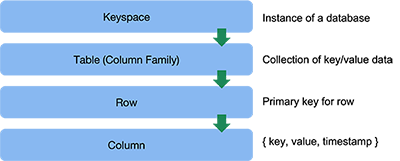
Table
Related rows are assembled into a table. A table is simply a container for these rows of data and is similar conceptually to tables in other databases. In the case of Bigtable, an instance of Bigtable had only one table. Cassandra supports the creation of multiple tables, where each row in the table is identified by a unique primary key as discussed in the previous section. This key is a collection of one or more columns.
Cassandra used to refer to collections of rows as a column family and this term is still present in much of the literature. Most likely, they avoided the term table to distinguish it from a relational database with its fixed columns. More recently, the project stopped using the term column family and switched to table.
Unlike relational databases, tables in the same Cassandra database are not related. There is no concept of foreign keys and no support for join queries where a query goes out and collects data from rows from multiple tables.
Because the location of each row in a table is determined by a hash of its partition key, different rows of a table may be located on different nodes. The collection of rows in a table that are located on the same machine are referred to as a partition. The collection of partitions across the nodes form the complete table. On each system, a partition is typically stored as a collection of files but the programmer need not be aware of the underlying storage structures. Each partition is replicated for fault tolerance.

To summarize, data is organized into tables. Each table is broken up into multiple partitions that are spread across the machines in the cluster. The partition key is the column whose value will be hashed to determine which machine stores that particular row (the partition key may be a composite key, in which case it will be a sequence of column names). Within each machine, a partition is sorted by clustering keys, which is a sequence of columns within the row. A primary key is the set of columns that will uniquely identify a row in the table. This is a partition key followed by zero or more clustering keys.
Keyspace
At the very top of the data hierarchy, and shared by all participating nodes, is a small chunk of information that defines how an instance of Cassandra behaves. This is called the keyspace. It can be thought of as a container of the tables for the database along with configuration such as the number of replicas and replication strategy.
Data storage
Now that we looked at the logical view of Cassandra’s data store, let’s look at how data flows in the system.
A client can contact any Cassandra node with a request. In most cases, clients are unaware of which nodes hold which partitions of a table. This node will act as the coordinator, forwarding the query to the appropriate node (or nodes), receiving the response, and returning it to the client. Cassandra uses the Apache Thrift RPC framework as a platform-neutral way to communicate.
Nodes in Cassandra exchange information about themselves and other nodes that they know about. In this way, knowledge of the cluster is propagated to all nodes. This information is timestamped with a vector clock, which allows nodes to ignore old versions of update messages. Note that this is the only place in Cassandra where vector clocks are used.
Cassandra spreads rows of tables across the cluster via a distributed hash table (DHT). The DHT is essentially the same design as the one used in Amazon Dynamo, which in turn is based on the Chord DHT. Systems are arranged in a logical ring and each node is responsible for a range of values. The coordinator applies a consistent hash function the partition key to generate a token. The request is then forwarded to the node whose range of hash values includes that token.
Just like Dynamo, Cassandra supports virtual nodes (vnodes) which allows each node to be configured to own multiple different hash ranges. This makes it easy to reconfigure the system to alleviate hot spots and to assign more vnodes to more powerful machines or machines with more storage.
The ring arrangement of nodes is also used for replications. Replicas are found by following the ring clockwise from the node that stores the initial replica.

Writes
Once the target node is identified and the request is forwarded by the coordinator, data writes (modifications or additions to a row) are handled in similar manner to Bigtable.
Data modifications are first written to a commit log in stable storage. This is an append-only log of changes. It provides durability in the event of system crashes by ensuring that the modification does not get lost even if the system crashes and restarts. On restart, any changes in the log will be applied on that node.
Next, the write operation is applied to an in-memory table called a memtable. This is a portion of the overall table partition on that node. A node has one active memtable per table. After this, the node sends back an acknowledgment that it received the request.
When the memtable reaches a certain size, it is written to the local file system as an SSTable (sorted string table). An SSTable stores a collection of rows for a table in the file system. It is implemented as a collection of files and is treated as a single object. These files include:
Data.db: the actual dataIndex.db: an index file of keysSummary.db: a sample of every 128th entry in the index fileFilter.db: a Bloom Filter of keys - an efficient structure to identify if a key is definitely not in the databaseCompressionInfo.db: stores offset information about compressed data in theData.dbfileStatistics.db: contains information about the Table, including timestamps, clustering keys, compression information, and time-to-live valuesDigest.crc32: a CRC-32 message digest used for integrity checkingTOC.txt: textual list of the files used for the SSTtable
The table partition is the collection of SSTables on this node. SSTables are immutable, which means that newer SSTables may make older ones obsolete, which will be deleted periodically.
Rows of data are sorted by the clustering keys and always remains sorted. Columns in a row are also kept sorted. Because of this, the naming of columns can impact system performance.
If the memtable contains multiple references to the same row (identical keys), only the most recent row will be written to the SSTable. Once data is written to the file, it is permanent and the commit log can be purged. Periodically, the node runs a process to merge SSTables for a given partition and key range and to remove stale SSTable files that are no longer needed.
Reads
Like writes, a read request is directed by the coordinator the the node that is responsible for that partition based on the partition key in the query. The requested data might be in the in-memory memtable if there were any recent modifications to that row. That data, though, may need to be merged with data that might be in one or more SSTable files.
To do this efficiently and avoid unnecessarily scanning SSTables, Cassandra stores a Bloom Filter for each SSTable. A Bloom Filter is an efficient hash-based structure that indicates if the desired data might be in the table or is definitely not in the table. Logically, you can think of it as a small hash table bitmap. Here we’re not using cryptographic hashes like the DHT does (which will typically return 128 or 256 bit values) but ons that return smaller results (the kind you’d use in a symbol table). You can hash a clustering key to get an index number. If the bitmap at that index is a 0 then it means that no key that hashes to this value exists in this table. If it’s a 1 then it means that the SSTable contains some key that hashes to this value so it might be the key we need.
If the required data might be in the SSTable then Cassandra will check an in-memory cache to find an index entry that will locate the partition summary. The partition summary will then contain the approximate location of the data. At that point, Cassandra will do a linear search for the desired row. The goal in this design is to keep the indexing structures small enough that they can be cached efficiently but minimize the number of disk reads that need to be done from the SSTables.
Replication
Since Cassandra is designed to be highly available, any data modifications will typically be replicated onto multiple nodes. Cassandra allows the programmer to define the replication factor – the number of copies of the row that will exist on multiple systems.
Writes are always sent by the coordinator to all replicas. The consistency level (see Replication, below) will determine the number of responses that the coordinator would need to get before responding to the client that issued the query.
The programmer also specifies a placement strategy. This tells Cassandra which nodes get the replicas. The first replica goes to the node determined by the hash of the partition key. The strategies supported include:
- Simple Strategy
- The entire cluster is treated as a collection of undifferentiated machines. Each replica is placed on the successor node in the DHT ring with no consideration of the location of the machine. This is a useful strategy when Cassandra is run in one data center in a single rack.
- Network Topology Strategy
- This is designed for deployments across data centers. An administrator specifies the replication parameters when creating the keyspace that include a sequenced list of data centers. It places replicas in the same data center by following the ring clockwise until it reaches the first successor node that is on a different rack. If a different data center is specified for one or more replicas, the ring is traversed clockwise until a successor node that resides at a different data center is located.
Tunable consistency
Cassandra provides eventual consistency. Cassandra’s replication is best-effort. This means that some replicas may have newer versions than others.
Like Dynamo, Cassandra can be configured to acknowledge client read or write requests based on the number of nodes that accepted these requests. This allows the programmer to decide on the tradeoff between consistency and availability.
Some predefined values include:
- ALL: All replicas must respond
- ONE, TWO, THREE: Only one, two, or three replicas must respond
- QUORUM: A majority of replicas must respond
- LOCAL_QUORUM: A majority of replicas in the local data center (where the coordinator is located) must respond
- EACH_QUORUM: A majority of replicas in each data center must respond
- ANY: No nodes need to acknowledge and the coordinator may store a hint and try later.
Conflicts and dead nodes
Cassandra does not use locks and does not enforce ACID semantics. It is possible for concurrent updates to create replicas with conflicting data. Amazon Dynamo used vector clocks to distinguish causal versus concurrent updates. Cassandra simply relies on timestamps and uses a last-write-wins approach. Every data mutation is timestamped, including deletions. The latest version of the data is treated as the winner.
It’s possible that the coordinator is unable to reach the desired node. If this happens and it needs to do a data modification, it stores a hinted handoff. This is a file of information about dead replicas it encountered and operations that need to be sent to them. Once a node discovers that a dead node has recovered, it goes through its list of hints and sends the request to the node. When it is acknowledged, the hint can be deleted.
Cassandra in use
After Facebook open-sourced Cassandra, it became an Apache project and has found use in over 7,000 companies. Some notable uses include:
- Apple has over 160,000 Cassandra nodes across 1,000+ clusters, storing 100 petabytes of data.
- Huawei has over 30,000 instances across 300+ clusters
- Netflix has over 10,000 instances across 100+ clusters with over 6 petabytes of data. Cassandra serves as the back-end database for streaming, processing over one trillion requests per day
- Discord uses it for storing messages – over 120M/day. All of its chat history is stored forever
- Uber stores data for live model predictions. Each driver & each customer sends location data every 30 seconds, resulting in over a million writes per second. In 2015, this was deployed on over 20 clusters and 300 machines
Cassandra is also used by companies that include Adobe, American Express, AT&T, eBay, HBO, Home Depot, Facebook, PayPal, Verizon, Target, Visa, Salesforce, Palantir, Spotify, and Weather Channel.
References
- Apache, Architecture, Cassandra Documentation.
- Apache, Data Types, Cassandra Documentation.
- Baeldung, Cassandra Partition Key, Composite Key, and Clustering Key, October 9, 2021.
- DataStax, How is the consistency level configured?, Apache Cassandra 3.0 documentation.
- DataStax, CQL Reference, Apache Cassandra 3.0 documentation.
- GeeksforGeeks, SSTable in Apache Cassandra, July 10, 2020.
- Google, Cloud Bigtable for Cassandra Users, Google Cloud – Cloud Architecture Center.
- Facebook (Meta), Cassandra – A structured storage system on a P2P Network. Engineering at Meta blog: describes the initial goals of Cassandra.
- Piyush Rana, Cassandra Data Modeling: Primary, Clustering, Partition, and Compound Keys, Database Zone (DZone), October 19, 2016.
- Christopher Sherman, Designing a Cassandra Data Model, Sherman Digital, April 26, 2017.
- Anup Shirolkar, A Comprehensive Guide to Cassandra Architecture, April 23, 2020.
- Sujith Jay Nair, Dynamo vs Cassandra : Systems Design of NoSQL Databases, Thinking Aloud blog, October 2, 2018.
-
We use the terms machine, node, system, computer, and server interchangeably. They all refer to a computer that’s running an instance of Cassandra and is part of the cluster of computers that runs the database. ↩︎
-
This isn’t a great example, since we could have simply used the state as the partition key. The only time we’d like to use a composite key in this case is if other countries had the same state names as the U.S. and we did not want to force them to be on the same machine as the U.S. states. ↩︎