Linear Algebra: Gaussian Elimination

Algorithm
OpenMP Implementation
MPI Implementation
CUDA Implementation

Algorithm

Gaussian elimination aims to transform a system of linear equations into an upper-triangular matrix in order to solve the unknowns and derive a solution. A pivot column is used to reduce the rows before it; then after the transformation, back-substitution is applied.

Example

Gaussian elimination is a method for solving matrix equations of the form

(1) To perform Gaussian elimination starting with the system of equations

(2) Compose the "augmented matrix equation"

(3) Here, the column vector in the variables X is carried along for labeling the matrix rows.
Now, perform elementary row operations to put the augmented matrix into the upper triangular form

(4) Solve the equation of the th row for , then substitute back into the equation of the (k-1)st row to
obtain a solution for Xk-1, etc., according to the formula

Example taken from:
http://mathworld.wolfram.com/GaussianElimination.html

Code

  for (int i = 0; i < N-1; i++) {
       for (int j = i; j < N; j++) {
           double ratio = A[j][i]/A[i][i];
           for (int k = i; k < N; k++) {
                A[j][k] -= (ratio*A[i][k]);
                b[j] -= (ratio*b[i]);
           }
       }
  }

OpenMP Implementation

Which Loops Are Parallelizable?
- Loops in which num of iterations known upon entry, and does not change.
- Loops in which each iteration independent of all others.
- Loops that contain no data dependence.
Observe the sequential code for Guassian Elimination provided above.
We have three possible candidate loops to parallelize. Which one should we select?
- First, we need to really understand how Gaussian Elimination works. This picture could help:
  
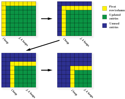
  (Picture taken from- http://riebecca.blogspot.com/2008/12/supercomputing-course-openmp-syntax-and_15.html)
  Gaussian elimination can be understood through the four frames of this picture, now we need to decide which loops to parallelize.
- The i loop is represented by the yellow row and column. The entries in the yellow row and column are being used to update the green sub matrix before going on to row/column i+1, meaning the values of the entries in the (i+1)st yellow area depend on what operations were performed on them at previous values of i. Therefore we can't use OpenMP to parallelize this loop because of data dependence.
- The j loop has a number of iterations that varies with i, but we do know the number of iterations every time we are about to enter the loop. None of the later iterations depend on the earlier ones and the iterations can be computed in any order! So the j loop is parallelizable.
- The k loop, like the j loop, has a number of iterations that varies but is calculable for every i. None of the later iterations depend on earlier ones, and they can all be computed in any order. Therefore the k loop is also parallelizable.
- It's best to select the outer loop (j), because then we'll have more uninterrupted parallelism and less forks and joins..
Gaussian Elimination using OpenMP:
  for (int i = 0; i < N-1; i++) {
  #pragma omp parallel for
       for (int j = i; j < N; j++) {
           double ratio = A[j][i]/A[i][i];
           for (int k = i; k < N; k++) {
                A[j][k] -= (ratio*A[i][k]);
                b[j] -= (ratio*b[i]);
           }
       }
  }

OpenMP Parallel Version of the Forward Elimination Algorithm

(This section is taken from- http://hpds.ee.kuas.edu.tw/download/parallel_processing/96/96present/20071212/Gaussian)

Code:

     do pivot = 1, (n-1)
  !$omp parallel do private(xmult) schedule(runtime)
       do i = (pivot+1), n
         xmult = a(i,pivot) / a(pivot,pivot)
         do j = (pivot+1), n
           a(i,j) = a(i,j) - (xmult * a(pivot,j))
         end do
         b(i) = b(i) - (xmult * b(pivot))
       end do
  !$omp end parallel do
     end do

With a static scheme and a specified chunk size, each processor is statically allocated chunk iterations. The allocation of iterations is done at the beginning of the loop, and each thread will only execute those iterations assigned to it. Using static without a specified chunk size implies the system default chunk size of n/p. Using a dynamic scheme, each thread is allocated a chunk of iterations at the beginning of the loop, but the exact set of iterations that are allocated to each thread is not known

Time Analysis:

MPI Implementation

root = 0
chunk = n**2/p 
! main loop
do pivot = 1, n-1
    ! root maintains communication            
    if (my_rank.eq.0) then
    ! adjust the chunk size
        if (MOD(pivot, p).eq.0) then
            chunk = chunk - n
        endif
        
        ! calculate chunk vectors
        rem = MOD((n**2-(n*pivot)),chunk)
        tmp = 0
        do i = 1, p
            tmp = tmp + chunk
            if (tmp.le.(n**2-(n*pivot))) then
                a_chnk_vec(i) = chunk
                b_chnk_vec(i) = chunk / n
            else
                a_chnk_vec(i) = rem
                b_chnk_vec(i) = rem / n
                rem = 0
            endif
        continue
        ! calculate displacement vectors
        a_disp_vec(1) = (pivot*n)
        b_disp_vec(1) = pivot
        do i = 2, p
            a_disp_vec(i) = a_disp_vec(i-1) 
                            + a_chnk_vec(i-1)
            b_disp_vec(i) = b_disp_vec(i-1) 
                            + b_chnk_vec(i-1)
            continue
            
            
            ! fetch the pivot equation
            do i = 1, n
                pivot_eqn(i) = a(n-(i-1),pivot)
            continue
            pivot_b = b(pivot)
        endif  ! my_rank.eq.0
        
        
    ! distribute the pivot equation
    call MPI_BCAST(pivot_eqn, n, 
                    MPI_DOUBLE_PRECISION,
                    root, MPI_COMM_WORLD, ierr)
    call MPI_BCAST(pivot_b, 1, 
                    MPI_DOUBLE_PRECISION,
                    root, MPI_COMM_WORLD, ierr)
                    
    ! distribute the chunk vector
    call MPI_SCATTER(a_chnk_vec, 1, MPI_INTEGER,
                    chunk, 1, MPI_INTEGER,
                    root, MPI_COMM_WORLD, ierr)
                    
    ! distribute the data
    call MPI_SCATTERV(a, a_chnk_vec, a_disp_vec, 
                        MPI_DOUBLE_PRECISION,
                        local_a, chunk, 
                        MPI_DOUBLE_PRECISION,
                        root, MPI_COMM_WORLD,ierr)
                        
    call MPI_SCATTERV(b, b_chnk_vec, b_disp_vec, 
                        MPI_DOUBLE_PRECISION,
                        local_b, chunk/n, 
                        MPI_DOUBLE_PRECISION,
                        root, MPI_COMM_WORLD,ierr)
                        
    ! forward elimination
    do j = 1, (chunk/n)
        xmult = local_a((n-(pivot-1)),j) / pivot_eqn(pivot)
        do i = (n-pivot), 1, -1
            local_a(i,j) = local_a(i,j) 
                     - (xmult * pivot_eqn(n-(i-1)))
        continue
        local_b(j) = local_b(j) - (xmult * pivot_b)
    continue
    
    ! restore the data to root
    call MPI_GATHERV(local_a, chunk, 
                        MPI_DOUBLE_PRECISION,
                        a, a_chnk_vec, a_disp_vec, 
                        MPI_DOUBLE_PRECISION,
                        root, MPI_COMM_WORLD, ierr)
    call MPI_GATHERV(local_b, chunk/n, 
                        MPI_DOUBLE_PRECISION,
                        b, b_chnk_vec, b_disp_vec, 
                        MPI_DOUBLE_PRECISION,
                        root, MPI_COMM_WORLD, ierr)
    continue ! end of main loop

http://hpds.ee.kuas.edu.tw/download/parallel_processing/96/96present/20071212/Gaussian.pdf

MPI parallel results using 2 processors
n	Communication Time	Workload Time	Total Time
400	2.15	0.72	2.88
800	18.28	5.76	24.03
1200	70.98	19.68	90.66

http://hpds.ee.kuas.edu.tw/download/parallel_processing/96/96present/20071212/Gaussian.pdf

Explanation: The above code is for forward elimination section of gaussian elimination.The matrix A and vector B are looped through and each equation is then set as a pivot. This pivot is then sent to each process as are the remaining pivot +1 to n equations. Process 0 is the master, it hhandles many aspects of the communication. MPI_ScatterV is used to distribute the data. Along with MPI_GatherV varing ammount of information can be distributed. MPI_Scatter is then used to distribute the chunk vector calculated from matrix A, (MPI_ScatterV cannot be used because each process does not know the chunk size beforehand, so instead of having them calculate this size MPI_Scatter is used). Matrix A has been distributed to create an even workload since as it's looped through the ammound of rows used decreases. Since fortran stored data sent/recieved by Scatterv in column-major order the algorithm is restructured to use this format and the data is reverted to row-major.

Since the ammount of time to perform the backwards substitution step is minimal when compared to the forward elimination it is best done sequentially.

The above tables show the time spend doing computations vs network communications for the forward elimination phase.

The most important aspect of Gaussian Elimination is communication times. Since the algorithm relies on so much data related work ( as opposed to task related) the communication time of the MPI non-shared memory implimentation vastly overshadows the workload time. Therefore this MPI solution is inferior to a shared-memory implimentation on the same machine.

CUDA Implementation

Code

This Gaussian Elimination example by Farhan Ahmad uses the standard algorithm with back-substitution to solve a linear system. It is implemented in C++ using standard CUDA C extensions. Data is read from a text file to load the matrices. You can view and download Ahmad's source code here.

main.cpp

#include<stdio.h>
#include<conio.h>
#include "Common.h"
#include<stdlib.h>

int main(int argc , char **argv) 
{ 
    float *a_h = NULL ;
    float *b_h = NULL ;
    float *result , sum ,rvalue ; 
    int numvar ,j ;

    numvar = 0; 

    // Reading the file to copy values 
    printf("\t\tShowing the data read from file\n\n"); 
    getvalue(&a_h , &numvar); 
    
    //Allocating memory on host for b_h 
    b_h = (float*)malloc(sizeof(float)*numvar*(numvar+1)); 
    
    //Calling device function to copy data to device 
    DeviceFunc(a_h , numvar , b_h); 
    
    //Showing the data 
    printf("\n\n"); 
    
    for(int i =0 ; i< numvar ;i++) 
    { 
        for(int j =0 ; j< numvar+1; j++) 
        { 
            printf("%f\n",b_h[i*(numvar+1) + j]); 
        } 
        printf("\n"); 
    } 

    //Using Back substitution method 
    result = (float*)malloc(sizeof(float)*(numvar)); 
    for(int i = 0; i< numvar;i++) 
    { 
        result[i] = 1.0;
    }

    for(int i=numvar-1 ; i>=0 ; i--) 
    { 
        sum = 0.0 ;

        for( j=numvar-1 ; j>i ;j--) 
        { 
            sum = sum + result[j]*b_h[i*(numvar+1) + j]; 
        }
        rvalue = b_h[i*(numvar+1) + numvar] - sum ; 
        result[i] = rvalue / b_h[i *(numvar+1) + j];
    } 
    
    //Displaying the result 
    printf("\n\t\tVALUES OF VARIABLES\n\n"); 
    for(int i =0;i<numvar;i++) 
    { 
        printf("[X%d] = %+f\n", i ,result[i]); 
    } 
    
    _getch(); 
    return 0; 
}

Kernel.cu

//Kernel function that executes on the device 
#include "Common.h" 
#include<cuda.h> 

__device__ __global__ void Kernel(float *a_d , float *b_d ,int size) 
{
    int idx = threadIdx.x ; 
    int idy = threadIdx.y ; 
    //int width = size ; 
    //int height = size ; 
    
    //Allocating memory in the share memory of the device 
    __shared__ float temp[16][16]; 
    
    //Copying the data to the shared memory 
    temp[idy][idx] = a_d[(idy * (size+1)) + idx] ; 
    
    for(int i =1 ; i<size ;i++) 
    { 
        if((idy + i) < size) // NO Thread divergence here 
        { 
            float var1 =(-1)*( temp[i-1][i-1]/temp[i+idy][i-1]); 
            temp[i+idy][idx] = temp[i-1][idx] +((var1) * (temp[i+idy ][idx]));
        } 
        __syncthreads(); //Synchronizing all threads before Next iterat ion 
    } 
    
    b_d[idy*(size+1) + idx] = temp[idy][idx]; 
}

DeviceFunc.cu

//Assigning memory on device and defining Thread Block size 
// Call to the Kernel(function) that will run on the GPU 

#include<cuda.h> 
#include<stdio.h> 
#include "Common.h" 

__device__ __global__ void Kernel(float *, float * ,int ); 

void DeviceFunc(float *temp_h , int numvar , float *temp1_h) 
{ 
    float *a_d , *b_d; 
    
    //Memory allocation on the device 
    cudaMalloc(&a_d,sizeof(float)*(numvar)*(numvar+1)); 
    cudaMalloc(&b_d,sizeof(float)*(numvar)*(numvar+1)); 
    
    //Copying data to device from host 
    cudaMemcpy(a_d, temp_h, sizeof(float)*numvar*(numvar+1),cudaMemcpyHostTo Device); 
    
    //Defining size of Thread Block 
    dim3 dimBlock(numvar+1,numvar,1); 
    dim3 dimGrid(1,1,1); 
    
    //Kernel call 
    Kernel<<<dimGrid , dimBlock>>>(a_d , b_d , numvar); 
    
    //Coping data to host from device 
    cudaMemcpy(temp1_h,b_d,sizeof(float)*numvar*(numvar+1),cudaMemcpyDeviceT oHost);

    //Deallocating memory on the device 
    cudaFree(a_d); 
    cudaFree(b_d); 
}

fread.cpp

//Reading from file 
#include<stdio.h> 
#include<stdlib.h> 
#include<math.h> 
#include<conio.h> 
#include "Common.h" 

void copyvalue(int , int * , FILE *,float*); // Function prototype
 
void getvalue(float **temp_h , int *numvar) { 
    FILE *data ; 
    int newchar ,index ; 

    index = 0; 

    data = fopen("B:\\data.txt","r"); 

    if(data == NULL) // if file does not exist 
    { 
        perror("data.txt"); 
        exit(1); 
    } 

    //First line contains number of variables 
    while((newchar = fgetc(data)) != '\n') 
    { 
        *numvar = (*numvar) * 10 + (newchar-48) ; 
    } 

    printf("\nNumber of variables = %d\n",*numvar);
    
    //Allocating memory for the array to store coefficients 
    *temp_h = (float*)malloc(sizeof(float)*(*numvar)*(*numvar+1));
    
    while(1) 
    { 
        //Reading the remaining data
        newchar = fgetc(data); 
        
        if(feof(data)) 
        { 
            break; '
        } 
        
        if(newchar == ' ') 
        {
            printf(" "); 
            continue; 
        } 
        else if(newchar == '\n') 
        { 
            printf("\n\n"); 
            continue; 
        } 
        else if((newchar >=48 && newchar <=57) newchar == '-')
        { 
            ungetc(newchar,data); 
            copyvalue(newchar,&index,data,*temp_h); 
        } 
        else { 
            printf("\nError:Unexpected symbol %c found",newchar);
            _getch(); 
            exit(1); 
        } 
    } 
} 

// copying the value from file to array 
void copyvalue(int newchar,int *i , FILE *data , float *temp_h) 
{ 
    float sum , sumfrac ; 
    double count ; 
    int ch; 
    int ptPresent = 0; 
    float sign; 
    
    sum = sumfrac = 0.0; 
    count = 1.0; 
    
    if(newchar == '-') 
    { 
        sign = -1.0; 
        fgetc(data); 
    } 
    else 
    { 
        sign = 1.0; 
    } 
    
    while(1) 
    { 
        ch = fgetc(data); 
        
        if(ch == '\n' ch == ' ') 
        { 
            ungetc(ch ,data); 
            break; 
        } 
        else if(ch == '.') 
        {
            ptPresent = 1; 
            break; 
        } 
        else 
        { 
            sum = sum*10 + ch-48; 
        } 
    } 
    
    if(ptPresent) 
    { 
        while(1) 
        { 
            ch = fgetc(data); 
            if(ch == ' ' ch == '\n') 
            { 
                ungetc(ch , data);
                break; 
            } 
            else 
            { 
                sumfrac = sumfrac + ((float)(ch-48))/pow(10.0,count);
                count++; 
            } 
        }
    } 
    
    temp_h[*i] = sign*(sum + sumfrac) ; 
    
    printf("[%f]",temp_h[*i]); 
    (*i)++; 
}

common.h

#ifndef __Common_H 
#define __Common_H 
#endif

void getvalue(float ** ,int *); 
void DeviceFunc(float * , int , float *);

The code is relatively straightforward. Because it is done in C++, the main function is compiled separately from the CUDA code. This portion of the program is run on the host's standard processor like a regular C++ program. It reads in the data from an external file. then transfers control to the device in DeviceFunc.cu. Here, memory is allocated and transferred from the main processor into the graphics processing unit. It prepares an execution configuration and then launches the kernel, which is the actual Gaussian Elimination code run in parallel by the GPU.

Other CUDA Implementations

Although the "typical" Gaussian elimination can be done in CUDA, several studies have found that there are more efficient ways of parallelizing the algorithm by making some adjustments. In one study by Xinggao Xia and Jong Chul Lee, rather than clearing only the rows before the pivot, all other rows are reduced to zero. Once each column is complete, no back-substitution is required. Partial pivoting is also used to ensure the accuracy of the answer.

In a different study by Aydin Buluc, John Gilbert, and Ceren Budak, they noted that while recursion is not possible on a CUDA GPU, it is on the host CPU. If recursion is used on the host, it separates the recursion stack from the floating-point operations done by the GPU, so that one does not interfere with the other. They use this so-called "recursive optimized" technique, along with other improvements like memory coalescing and optimized primitive variables in order to attain maximum speedup.

Xia and Lee's presentation can be found here.
Buluc et. al.'s paper on different Gaussian-Elimination style algorithms for GPGPU can be found here.

Linear Algebra: Gaussian Elimination

Contents

Algorithm

Example

Code

OpenMP Implementation

OpenMP Parallel Version of the Forward Elimination Algorithm

MPI Implementation

CUDA Implementation

Code

main.cpp

Kernel.cu

DeviceFunc.cu

fread.cpp

common.h

Other CUDA Implementations