Which Digit?
 |
 |
 |
 |
 |
 |
 |
 |
 |
 |
 |
 |
 |
 |
 |
| Which Digit? |
|
In this project, you will design three classifiers: a naive Bayes classifier, a perceptron classifier and a large-margin (MIRA) classifier. You will test your classifiers on two image data sets: a set of scanned handwritten digit images and a set of face images in which edges have already been detected. Even with simple features, your classifiers will be able to do quite well on these tasks when given enough training data.
Optical character recognition (OCR) is the task of extracting text from image sources. The first data set on which you will run your classifiers is a collection of handwritten numerical digits (0-9). This is a very commercially useful technology, similar to the technique used by the US post office to route mail by zip codes. There are systems that can perform with over 99% classification accuracy (see LeNet-5 for an example system in action).
Face detection is the task of localizing faces within video or still images. The faces can be at any location and vary in size. There are many applications for face detection, including human computer interaction and surveillance. You will attempt a simplified face detection task in which your system is presented with an image that has been pre-processed by an edge detection algorithm. The task is to determine whether the edge image is a face or not. There are several systems in use that perform quite well at the face detection task. One good system is the Face Detector by Schneiderman and Kanade. You can even try it out on your own photos in this demo.
The code for this project includes the following files and data, available as a zip file.
Data file |
|
data.zip |
Data file, including the digit and face data. |
Files you will edit |
|
naiveBayes.py |
The location where you will write your naive Bayes classifier. |
perceptron.py |
The location where you will write your perceptron classifier. |
mira.py |
The location where you will write your MIRA classifier. |
dataClassifier.py |
The wrapper code that will call your classifiers. You will use this code to analyze the behavior of your classifier and may edit some parts of it if you want to. |
answers.py |
Answers to Question 2 and Question 4 go here. |
Files you should read but NOT edit |
|
classificationMethod.py |
Abstract super class for the classifiers you will write. (You should read this file carefully to see how the infrastructure is set up.) |
samples.py |
I/O code to read in the classification data. |
util.py |
Code defining some useful tools. You may be familiar with some of these by now, and they will save you a lot of time. |
mostFrequent.py |
A simple baseline classifier that just labels every instance as the most frequent class. |
runMinicontest.py |
The command you will use to run the minicontest, if you decide to enter. |
What to submit: You will fill in portions of answers.py,
naiveBayes.py, perceptron.py,
mira.py and dataClassifier.py
(only) during the assignment, and submit them.
Evaluation: Your code will be autograded for technical correctness. Please do not change the names of any provided functions or classes within the code, or you will wreak havoc on the autograder.
Academic Dishonesty: We will be checking your code against other submissions in the class for logical redundancy. If you copy someone else's code and submit it with minor changes, we will know. These cheat detectors are quite hard to fool, so please don't try. We trust you all to submit your own work only; please don't let us down. Instead, contact the course staff if you are having trouble.
To try out the classification pipeline, run dataClassifier.py
from the command line. This will classify the digit data using the default
classifier (mostFrequent) which blindly classifies every
example with the most frequent label.
python dataClassifier.py
As usual, you can learn more about the possible command line options by running:
python dataClassifier.py -h
We have defined some simple features for you. Later you will design some
better features. Our simple feature set includes one feature for each
pixel location, which can take values 0 or 1 (off or on). The features are
encoded as a Counter where keys are feature locations
(represented as (column,row)) and values are 0 or 1. The face recognition
data set has value 1 only for those pixels identified by a Canny edge
detector.
Implementation Note: You'll find it easiest to hard-code the binary feature assumption. If you do, make sure you don't include any non-binary features. Or, you can write your code more generally, to handle arbitrary feature values, though this will probably involve a preliminary pass through the training set to find all possible feature values (and you'll need an "unknown" option in case you encounter a value in the test data you never saw during training).
A skeleton implementation of a naive Bayes classifier is provided for
you in naiveBayes.py. You
will fill in the trainAndTune function, the calculateLogJointProbabilities
function and the findHighOddsFeatures function.
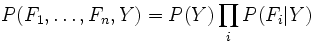
A naive Bayes classifier models a joint distribution over a label ![]() and a set of observed random variables, or features,
and a set of observed random variables, or features, ![]() ,
using the assumption that the full joint distribution can be factored as
follows (features are conditionally independent given the label):
,
using the assumption that the full joint distribution can be factored as
follows (features are conditionally independent given the label):
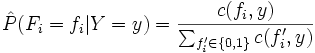
To classify a datum, we can find the most probable label given the feature values for each pixel, using Bayes theorem:
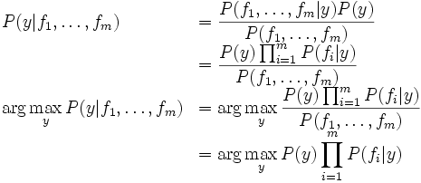
Because multiplying many probabilities together often results in underflow, we will instead compute log probabilities which have the same argmax:

To compute logarithms, use math.log(), a built-in Python
function.
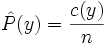
We can estimate ![]() directly from the training data:
directly from the training data:
The other parameters to estimate are the conditional
probabilities of our features given each label y: ![]() .
We do this for each possible feature value (
.
We do this for each possible feature value (![]() ).
).
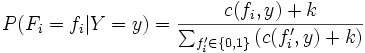
In this project, we use Laplace smoothing, which adds k counts to every possible observation value:
If k=0, the probabilities are unsmoothed. As k grows larger, the probabilities are smoothed more and more. You can use your validation set to determine a good value for k. Note: don't smooth P(Y).
Question 1 (6 points) Implement trainAndTune
and calculateLogJointProbabilities in naiveBayes.py.
In trainAndTune, estimate conditional probabilities from the
training data for each possible value of k given in the list kgrid.
Evaluate accuracy on the held-out validation set for each k and
choose the value with the highest validation accuracy. In case of ties,
prefer the lowest value of k. Test your classifier
with:
python dataClassifier.py -c naiveBayes --autotune
Hints and observations:
calculateLogJointProbabilities uses the
conditional probability tables constructed by trainAndTune
to compute the log posterior probability for each label y given a
feature vector. The comments of the method describe the data structures
of the input and output. analysis method in dataClassifier.py
to explore the mistakes that your classifier is making. This is
optional. --autotune option. This will ensure that kgrid
has only one value, which you can change with -k. --autotune, which tries different values of k,
you should get a validation accuracy of about 74% and a test accuracy of
65%. Counter.argMax()
method. -d faces
(optional). Another, better, tool for understanding the parameters is to look at odds
ratios. For each pixel feature ![]() and classes
and classes ![]() ,
consider the odds ratio:
,
consider the odds ratio:
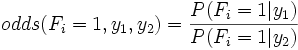
The features that have the greatest impact at classification time are those with both a high probability (because they appear often in the data) and a high odds ratio (because they strongly bias one label versus another).
To run the autograder for this question:
python autograder.py -q q1
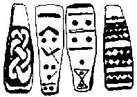
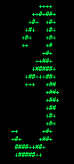
Question 2 (2 points) Fill in the function findHighOddsFeatures(self,
label1, label2). It should return a list of the 100 features with
highest odds ratios for label1 over label2.
The option -o activates an odds ratio analysis. Use the
options -1 label1 -2 label2 to specify which labels to
compare. Running the following command will show you the 100 pixels that
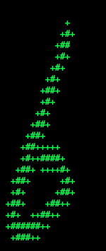
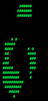
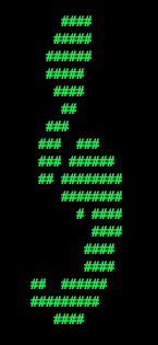
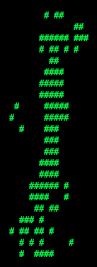
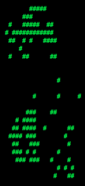
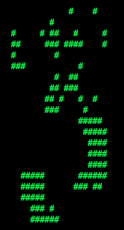
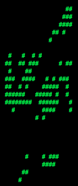
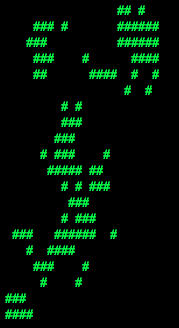
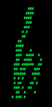
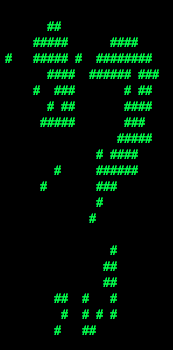
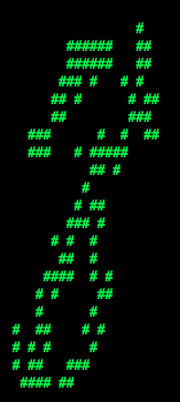
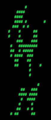
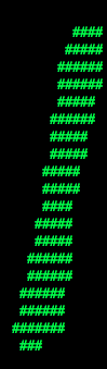
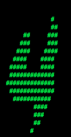
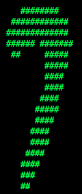
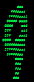
best distinguish between a 3 and a 6.
python dataClassifier.py -a -d digits -c naiveBayes -o -1 3 -2 6Use what you learn from running this command to answer the following question. Which of the following images best shows those pixels which have a high odds ratio with respect to 3 over 6? (That is, which of these is most like the output from the command you just ran?)
 |
 |
 |
 |
 |
|
|
|
|
|
|
To answer: please return 'a', 'b', 'c', 'd', or 'e' from the
function q2 in answers.py.
Hints:
perceptron.py. You will fill
in the train function, and the findHighWeightFeatures
function.
Unlike the naive Bayes classifier, a perceptron does not use
probabilities to make its decisions. Instead, it keeps a weight vector ![]() of each class
of each class ![]() (
(![]() is an identifier, not an exponent). Given a feature list
is an identifier, not an exponent). Given a feature list ![]() ,
the perceptron compute the class
,
the perceptron compute the class ![]() whose weight vector is most similar to the input vector
whose weight vector is most similar to the input vector ![]() .
Formally, given a feature vector
.
Formally, given a feature vector ![]() (in our case, a map from pixel locations to indicators of whether they are
on), we score each class with:
(in our case, a map from pixel locations to indicators of whether they are
on), we score each class with:
Counter.
Using the addition, subtraction, and multiplication functionality of the
Counter class in util.py,
the perceptron updates should be relatively easy to code. Certain
implementation issues have been taken care of for you in perceptron.py,
such as handling iterations over the training data and ordering the update
trials. Furthermore, the code sets up the weights data
structure for you. Each legal label needs its own Counter
full of weights.
Question 3 (4 points) Fill in the train
method in perceptron.py.
Run your code with:
python dataClassifier.py -c perceptron
Hints and observations:
-i
          iterations
option. Try different numbers of iterations and see
how it influences the performance. In practice, you would use the
performance on the validation set to figure out when to stop training,
but you don't need to implement this stopping criterion for this
assignment.To run the autograder for this question and visualize the output:
python autograder.py -q q3
Perceptron classifiers, and other discriminative methods, are often criticized because the parameters they learn are hard to interpret. To see a demonstration of this issue, we can write a function to find features that are characteristic of one class. (Note that, because of the way perceptrons are trained, it is not as crucial to find odds ratios.)
Question 4 (1 point) Fill in findHighWeightFeatures(self,
label) in perceptron.py.
It should return a list of the 100 features with highest weight for that
label. You can display the 100 pixels with the largest weights using the
command:
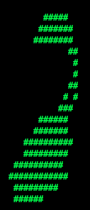
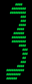
python dataClassifier.py -c perceptron -wUse this command to look at the weights, and answer the following true/false question. Which of the following sequence of weights is most representative of the perceptron?
| (a) | 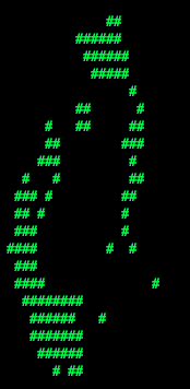 |
 |
 |
 |
 |
 |
 |
 |
 |
 |
| (b) |  |
 |
 |
 |
 |
 |
 |
 |
 |
 |
answers.py
in the method q4, returning either 'a' or 'b'.
mira.py.
MIRA is an online learner which is closely related to both the support
vector machine and perceptron classifiers. You will fill in the trainAndTune
function.
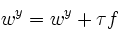
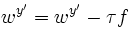
 is chosen such that it minimizes
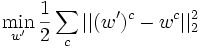
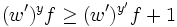
 subject to
 and
and
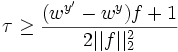
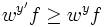 , so the condition
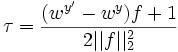
is always true given Solving
this simple problem, we then have
, so the condition
is always true given Solving
this simple problem, we then have
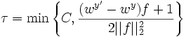
 by a positive constant C, which leads us to
trainAndTune
in mira.py. This method should
train a MIRA classifier using each value of C in Cgrid.
Evaluate accuracy on the held-out validation set for each C and
choose the C with the highest validation accuracy. In case of
ties, prefer the lowest value of C. Test your MIRA
implementation with:
python dataClassifier.py -c mira --autotune
Hints and observations:
self.max_iterations times during
training. self.weights, so that these weights can be used to
test your classifier. --autotune
option from the command above. --autotune
should be in the 60's. To run the autograder for this question and visualize the output:
python autograder.py -q q5
Congratulations! You're finished all projects.